Pipeline Parallelism: Surgery on Models Too Big for the Operating Table

In our latest article, we explored Data Parallelism. While this parallelization technique clearly boosts training efficiency and resource utilization, it has a fundamental limitation: it doesn’t help us train larger models or reduce the hardware footprint of a single model. So what do we do when faced with a truly massive model? How do we train something that simply refuses to fit on a single GPU?

Enter model parallelism. Today, we’re diving into a specific technique called Pipeline Parallelism. I’m starting here because, at first glance, it’s the most intuitive approach. But don’t be fooled by its apparent simplicity. Pipeline Parallelism is full of hidden complexities and clever tricks that only reveal themselves once you dig deeper.

The Basic Idea

Pipeline Parallelism works by surgically dividing your model into groups of consecutive layers, then distributing these groups across your available GPUs. Picture an LLM with 16 layers and 8 GPUs at your disposal. You’d assign layers 1-2 to GPU_0, layers 3-4 to GPU_1, layers 5-6 to GPU_2, and continue this pattern. The goal? Balance the computational workload evenly. Each GPU ends up hosting exactly 2 layers.

$$\text{layers_per_gpu} = \frac{\text{n_layers}}{\text{n_gpus}}$$

Most frameworks actually enforce this even distribution. Try to assign an uneven number of layers per GPU, and you’ll likely hit a wall (unless you’re willing to get your hands dirty with custom modifications).

The Naive Approach (and Why It’s Terrible)

How does a single batch flow through this setup? First, it passes through GPU_0’s layers, then moves to GPU_1’s layers, then GPU_2’s, and so on. During backpropagation, we reverse direction. In a 4-GPU setup, it looks like this:

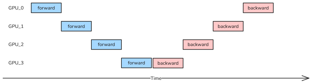
Notice that in reality, the backward pass takes more time than the forward step, therefore the idle time for GPU_0 would be even greater.

Now, if you’re thinking “that looks inefficient,” you’re absolutely right. This naive implementation is a disaster. Each GPU sits idle for approximately (100 - 100/n_gpus)% of the time.

Let’s diagnose what’s happening to GPU_0: After completing its forward pass, it enters a waiting room. It waits for GPU_1 to finish. Then GPU_2. Then GPU_3. Finally, all the forward passes complete. But it’s not done waiting! Now it watches as GPU_3 does its backward pass, then GPU_2, then GPU_1. Only then can GPU_0 finally perform its own backward pass.

Do the math: GPU_0 is actively working only 25% of the time. It’s like having a highly-skilled surgeon who spends 45 minutes of every hour sitting in the break room while a single operation moves through different stages. The inefficiency is staggering and completely unacceptable.

Microbatching to the Rescue

We can salvage this approach by splitting our input batch into smaller micro-batches. Now, GPU_0 doesn’t sit idle after processing microbatch_0’s forward pass. Instead, it immediately moves on to microbatch_1, then microbatch_2, and so forth. Here’s what this looks like:

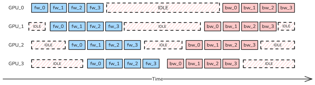
Better, right? But notice those IDLE blocks haven’t disappeared. In pipeline parallelism terminology, we call these bubbles, and they represent the dead time each GPU spends waiting during the training pipeline. The good news? We can actually calculate the size of these bubbles with some straightforward math.

Let’s start by defining the time each GPU needs to process one micro-batch. This is simply the sum of its forward and backward passes:

$$t_g = t_f + t_b$$

Now, think back to our first example without micro-batching. GPU_0 had to wait for all the other GPUs to finish their work. We can express this waiting time as:

$$t_w = (p-1) \cdot (t_f + t_b)$$

The (P-1) term represents the degree of parallelism minus one. Since this waiting pattern applies to every GPU in our pipeline, we can compute the bubble time as the ratio of waiting time to processing time:

$$t_{\text{bubble}} = \frac{t_w}{t_g} = p - 1$$

Notice something concerning? As we add more pipeline stages, the bubble time grows. Not ideal.

With micro-batching, each GPU processes N micro-batches instead of one large batch. This multiplies the total GPU processing time by a factor of N:

$$t_{\text{bubble}} = \frac{t_w}{N \cdot t_g} = \frac{p-1}{N}$$

Beautiful! We’re reducing the bubble time by a factor of N. The more micro-batches, the smaller those wasteful idle periods become.

As we know all too well, there’s no free lunch. Micro-batching demands more memory because we must store the activations for each micro-batch until we reach its corresponding backward pass. This is a critical point: Pipeline Parallelism won’t help you reduce activation memory. If you’re hitting out-of-memory errors because of activations, PP alone won’t save you. Keep this in mind when diagnosing memory issues.

You might think, “Why not take this to the extreme and set micro-batch size to 1?”. That’s actually a great idea, because that would minimize the activation storage burden. However, that won’t reduce the duration of the bubbles because, it would still be proportional to the number of pipeline stages, as stated in the formula above.

Interleaving Schedules

So how else can we shrink those bubbles? Let’s rethink our entire approach. Up to now, we’ve operated under a simple assumption: each rank hosts a contiguous block of layers. Rank_0 gets layers 0-3, rank_1 gets layers 4-7, and so on. It’s clean, intuitive, and straightforward.

But what if we got creative with our layer assignment? Instead of contiguous blocks, we could give each rank a scattered, heterogeneous collection of layers. The key insight: for any given micro-batch’s forward pass, each rank would execute multiple pipeline stages instead of just one.

Here’s a concrete example. Imagine assigning layers using a modulo scheme based on the number of ranks. With 4 GPUs, rank_0 would host layers 0, 4, 8, 12, ..., while rank_1 would take layers 1, 5, 9, 13, ..., and so forth. Now each rank participates multiple times as data flows through the model.

This interleaved approach changes our bubble calculation fundamentally. We need to account for the fact that both forward and backward passes are now divided across multiple visits to each GPU. We introduce a factor v representing the number of model chunks per GPU (equivalently, the number of times a GPU is visited per micro-batch). The bubble formula becomes:

$$t_{\text{bubble}} = \frac{1}{v} \cdot \frac{(p-1) \cdot (t_f + t_b)}{N \cdot (t_f + t_b)} = \frac{p-1}{v \cdot N}$$

The bubble duration still grows with the number of pipeline stages (P), but now it’s inversely proportional to both the number of micro-batches (N) and the number of model chunks per GPU (v). We’ve added another lever to pull for reducing those wasteful idle periods.

Predictably, this cleverness comes with costs. Scattering layers across GPUs increases communication overhead. Data must hop between ranks more frequently, and each hop burns precious time. Additionally, the scheduling logic becomes significantly more complex. The pipeline scheduler, which was already juggling microbatches, now has to coordinate these interleaved layer executions without creating deadlocks or bottlenecks.

Finding the optimal configuration for a given model and parallelization setup? Unfortunately, it’s still largely trial and error. For tasks like this, I recommend deploying the most reliable optimization algorithm we have: graduate student descent.

More Sophisticated Approaches

Recently, two innovative approaches have emerged to push the boundaries of bubble reduction even further. ZeroBubble was proposed by Sea AI Lab, and DualPipe, which builds upon it, came from DeepSeek.

ZeroBubble: Rethinking the Backward Pass

ZeroBubble’s central insight is elegantly simple: the backward pass isn’t actually monolithic. It consists of two distinct stages. First, there’s the backward computation for the inputs, which the authors call B. Second, there’s the backward computation for the weights, which they call W.

Here’s where it gets interesting. Consider an arbitrary layer L in your architecture. When computing the backward pass for layer L+1 (the layer below L in the pipeline), that computation depends only on B, not on W. This dependency structure reveals a crucial opportunity: W can be computed at any point after B completes and before the optimizer step runs.

The ZeroBubble authors exploit this flexibility strategically. Instead of computing W immediately after B (as traditional schedules do), they defer W computations and slot them into those otherwise wasted bubble periods. It’s like finding useful prep work for a surgeon to do during what would otherwise be idle time between patients.

DualPipe: Bidirectional Scheduling

DualPipe takes these ideas further with a genuinely innovative approach. Its defining feature is bidirectional scheduling, which fundamentally reimagines how micro-batches flow through the pipeline.

Traditional pipeline parallelism feeds micro-batches through in one direction, from the first layer to the last. DualPipe breaks this pattern by injecting micro-batches from both ends of the pipeline simultaneously, creating dual channels of execution.

This bidirectional design has profound implications. A single GPU (pipeline stage) can now handle forward passes for micro-batches arriving from one direction while simultaneously processing backward passes for micro-batches coming from the opposite direction. This overlapping execution dramatically increases GPU utilization and slashes bubble time even further.

However, supporting this bidirectional flow requires a trade-off. Each GPU must hold copies of its model layers for both directions, leading to parameter redundancy. In practice, this typically doubles the memory footprint compared to single-direction pipelines like ZeroBubble. The increased memory usage is the price you pay for those efficiency gains, though subsequent research has explored optimized variations of DualPipe that reduce this redundancy.

Wrapping Up

Pipeline Parallelism gives us a practical way to train models that simply won’t fit on a single GPU. By distributing layers across devices and cleverly micro-batching our data, we can keep those GPUs busy and make training feasible. The bubbles never completely disappear, but with techniques like interleaved schedules, ZeroBubble, and DualPipe, we’ve gotten pretty good at minimizing them.

I hope you enjoyed this first dive into model parallelism. Next time, we’ll explore another dimension of this fascinating puzzle. See you then!